Travelling Salesman Problem – Solved using Branch and Bound
Travelling Salesman Problem – What it is?
- Travelling Salesman Problem (TSP) is an interesting problem. Problem is defined as “given n cities and distance between each pair of cities, find out the path which visits each city exactly once and come back to starting city, with the constraint of minimizing the travelling distance.”
- TSP has many practical applications. It is used in network design, and transportation route design. The objective is to minimize the distance. We can start tour from any random city and visit other cities in any order. With n cities, n! different permutations are possible. Exploring all paths using brute force attacks may not be useful in real life applications.
LCBB using Static State Space Tree for Travelling Salseman Problem
- Branch and bound is an effective way to find better, if not best, solution in quick time by pruning some of the unnecessary branches of search tree.
- It works as follow :
Consider directed weighted graph G = (V, E, W), where node represents cities and weighted directed edges represents direction and distance between two cities.
1. Initially, graph is represented by cost matrix C, where
Cij = cost of edge, if there is a direct path from city i to city j
Cij = ∞, if there is no direct path from city i to city j.
2. Convert cost matrix to reduced matrix by subtracting minimum values from appropriate rows and columns, such that each row and column contains at least one zero entry.
3. Find cost of reduced matrix. Cost is given by summation of subtracted amount from the cost matrix to convert it in to reduce matrix.
4. Prepare state space tree for the reduce matrix
5. Find least cost valued node A (i.e. E-node), by computing reduced cost node matrix with every remaining node.
6. If <i, j> edge is to be included, then do following :
(a) Set all values in row i and all values in column j of A to ∞
(b) Set A[j, 1] = ∞
(c) Reduce A again, except rows and columns having all ∞ entries.
7. Compute the cost of newly created reduced matrix as,
Cost = L + Cost(i, j) + r
Where, L is cost of original reduced cost matrix and r is A[i, j].
8. If all nodes are not visited then go to step 4.
Reduction procedure is described below :
Raw Reduction:
Matrix M is called reduced matrix if each of its row and column has at least one zero entry or entire row or entire column has ∞ value. Let M represents the distance matrix of 5 cities. M can be reduced as follow:
MRowRed = {Mij – min {Mij | 1 ≤ j ≤ n, and Mij < ∞ }}
Consider the following distance matrix:

Find the minimum element from each row and subtract it from each cell of matrix.

Reduced matrix would be:

Row reduction cost is the summation of all the values subtracted from each rows:
Row reduction cost (M) = 10 + 2 + 2 + 3 + 4 = 21
Column reduction:
Matrix MRowRed is row reduced but not the column reduced. Matrix is called column reduced if each of its column has at least one zero entry or all ∞ entries.
MColRed = {Mji – min {Mji | 1 ≤ j ≤ n, and Mji < ∞ }}
To reduced above matrix, we will find the minimum element from each column and subtract it from each cell of matrix.

Column reduced matrix MColRed would be:

Each row and column of MColRed has at least one zero entry, so this matrix is reduced matrix.
Column reduction cost (M) = 1 + 0 + 3 + 0 + 0 = 4
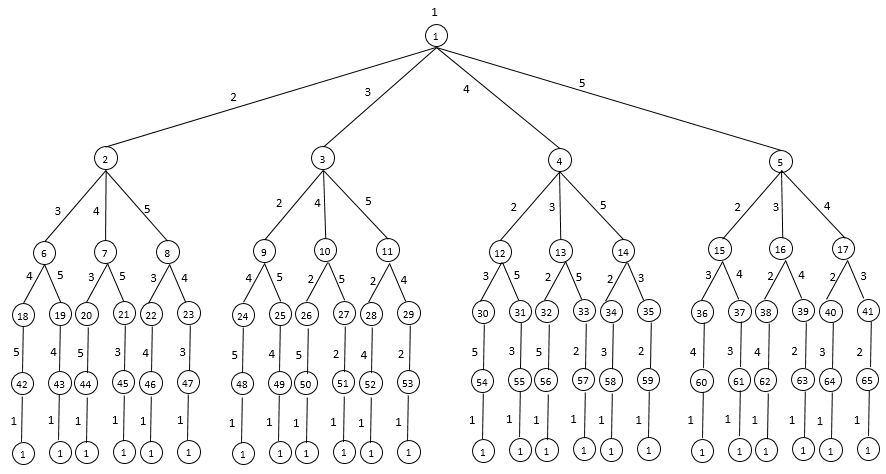
State space tree for 5 city problem is depicted in Fig. 6.6.1. Number within circle indicates the order in which the node is generated, and number of edge indicates the city being visited.
Example
Example: Find the solution of following travelling salesman problem using branch and bound method.

Solution:
- The procedure for dynamic reduction is as follow:
- Draw state space tree with optimal reduction cost at root node.
- Derive cost of path from node i to j by setting all entries in ith row and jth column as ∞.
Set M[j][i] = ∞
- Cost of corresponding node N for path i to j is summation of optimal cost + reduction cost + M[j][i]
- After exploring all nodes at level i, set node with minimum cost as E node and repeat the procedure until all nodes are visited.
- Given matrix is not reduced. In order to find reduced matrix of it, we will first find the row reduced matrix followed by column reduced matrix if needed. We can find row reduced matrix by subtracting minimum element of each row from each element of corresponding row. Procedure is described below:
- Reduce above cost matrix by subtracting minimum value from each row and column.

\[ M_{1}^{‘} \] is not reduced matrix. Reduce it subtracting minimum value from corresponding column. Doing this we get,

Cost of M1 = C(1)
= Row reduction cost + Column reduction cost
= (10 + 2 + 2 + 3 + 4) + (1 + 3) = 25
This means all tours in graph has length at least 25. This is the optimal cost of the path.
State space tree

Let us find cost of edge from node 1 to 2, 3, 4, 5.
Select edge 1-2:
Set M1 [1] [ ] = M1 [ ] [2] = ∞
Set M1 [2] [1] = ∞
Reduce the resultant matrix if required.

M2 is already reduced.
Cost of node 2 :
C(2) = C(1) + Reduction cost + M1 [1] [2]
= 25 + 0 + 10 = 35
Select edge 1-3
Set M1 [1][ ] = M1 [ ] [3] = ∞
Set M1 [3][1] = ∞
Reduce the resultant matrix if required.

Cost of node 3:
C(3) = C(1) + Reduction cost + M1[1] [3]
= 25 + 11 + 17 = 53
Select edge 1-4:
Set M1 [1][ ] = M1[ ][4] = ∞
Set M1 [4][1] = ∞
Reduce resultant matrix if required.

Matrix M4 is already reduced.
Cost of node 4:
C(4) = C(1) + Reduction cost + M1 [1] [4]
= 25 + 0 + 0 = 25
Select edge 1-5:
Set M1 [1] [ ] = M1 [ ] [5] = ∞
Set M1 [5] [1] = ∞
Reduce the resultant matrix if required.

Cost of node 5:
C(5) = C(1) + reduction cost + M1 [1] [5]
= 25 + 5 + 1 = 31
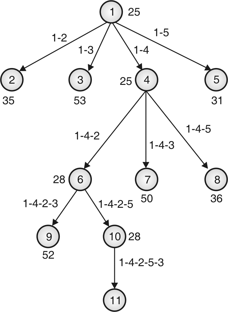
State space diagram:

Node 4 has minimum cost for path 1-4. We can go to vertex 2, 3 or 5. Let’s explore all three nodes.
Select path 1-4-2 : (Add edge 4-2)
Set M4 [1] [] = M4 [4] [] = M4 [] [2] = ∞
Set M4 [2] [1] = ∞
Reduce resultant matrix if required.

Matrix M6 is already reduced.
Cost of node 6:
C(6) = C(4) + Reduction cost + M4 [4] [2]
= 25 + 0 + 3 = 28
Select edge 4-3 (Path 1-4-3):
Set M4 [1] [ ] = M4 [4] [ ] = M4 [ ] [3] = ∞
Set M [3][1] = ∞
Reduce the resultant matrix if required.

\[ M_{7}^{‘} \] is not reduced. Reduce it by subtracting 11 from column 1.

Cost of node 7:
C(7) = C(4) + Reduction cost + M4 [4] [3]
= 25 + 2 + 11 + 12 = 50
Select edge 4-5 (Path 1-4-5):

Matrix M8 is reduced.
Cost of node 8:
C(8) = C(4) + Reduction cost + M4 [4][5]
= 25 + 11 + 0 = 36
State space tree
Path 1-4-2 leads to minimum cost. Let’s find the cost for two possible paths.

Add edge 2-3 (Path 1-4-2-3):
Set M6 [1][ ] = M6 [4][ ] = M6 [2][ ]
= M6 [][3] = ∞
Set M6 [3][1] = ∞
Reduce resultant matrix if required.


Cost of node 9:
C(9) = C(6) + Reduction cost + M6 [2][3]
= 28 + 11 + 2 + 11 = 52
Add edge 2-5 (Path 1-4-2-5):
Set M6 [1][ ] = M6 [4][ ] = M6 [2][ ] = M6 [ ][5] = ∞
Set M6 [5][1] = ∞
Reduce resultant matrix if required.

Cost of node 10:
C(10) = C(6) + Reduction cost + M6 [2][5]
= 28 + 0 + 0 = 28
State space tree

Add edge 5-3 (Path 1-4-2-5-3):

Cost of node 11:
C(11) = C(10) + Reduction cost + M10 [5][3]
= 28 + 0 + 0 = 28
State space tree:
LCBB using Dynamic State Space Tree
- Static space tree is m-ary tree. In dynamic state space tree, left and right branch indicates inclusion and exclusion of edge respectively. Bounding function computation is same as previous method. Dynamic state space tree is binary tree. At each node, left branch (i, j) indicates all the paths including edge (i, j). Right branch (i, j) indicates all the paths excluding (i, j).
- At each level, we select the edge which gives highest probability of minimum tour cost. This can be done by selecting the right edge which gives highestvalue. We can find such edge from reduced cost matrix. Consider the following instance of TSP.


- Reduced matrix is computed in same way, as we did in previous case. Reduction cost of the matrix is 25. This implies, any route of the graph costs at least 25. Thus root of the tree has cost 25. We shall select the next edge such that exclusion of that leads to maximum. In other words, select the edge which gives maximum probability of minimum cost of path on inclusion of that edge.
- We can achieve this by considering one of the edge with reduced cost zero in reduced matrix. In
Fig. 6.6.2(b) edge <1, 4>, <2, 5>, <3, 1>, <3, 4>, <4, 5>, <5, 2> and <5, 3> has 0 reduction cost. If we select any of the edge <a, b> from this list, then resultant cost matrix M will have entry ∞ on position M[a][b]. - If we include edge <1, 4>, set M[1][4] = ∞, and reduce M. This is done by subtracting 1 from row 1. So cost of right child will increase by 1.
- If we include edge <2, 5>, set M[2][5] = ∞, and reduce M. This is done by subtracting 2 from row 2. So cost of right child will increase by 1.
- If we include edge <3, 1>, set M[3][1] = ∞, and reduce M. This is done by subtracting 11 from column 1. So cost of right child will increase by 11.
Thus we will have,
| Edge | <1, 4> | <2, 5> | <3, 1> | <3, 4> | <4, 5> | <5, 2> | <5, 3> |
| Increment in \[ hat{c} \] of right child | 1 | 2 | 11 | 0 | 3 | 3 | 11 |
Here, edge <3, 1> and <5, 3> maximizes the cost of right child, so we can select any one of them. Let us select edge <3, 1>.

Cost of matrix M2= Cost of node 2, C(2)
= C(1) + L + M[3][1] = 25 + 0 + 0 = 25
By excluding <3, 1> we get,

Cost of matrix M3 = Cost of node 3,
C(3) = C(1) + L + M[3][1] = 25 + 11 + 0 = 36
At this point, dynamic state space tree would look like,

On inclusion of <3, 1>, we get matrix M2. In M2, we have <1, 4>, <2, 5>, <4, 5>, <5, 2> and <5, 3> edges with 0 value. So selecting any of the edge <a, b> from this list will make M2[a][b] = ∞. Repeating previous step, we get
| Edge | <1, 4> | <2, 5> | <4, 5> | <5, 2> | <5, 3> |
| Increment in \[ hat{c} \] of right child | 3 | 2 | 3 | 3 | 11 |
Here, edge <5, 3> maximizes of right child, so let us select edge <5, 3>.

Cost of matrix M4= Cost of node 4,
C(4) = C(2) + L + M2[5][3] = 25 + 3 + 0 = 28
By excluding <5, 3> we get,

Cost of matrix M5= Cost of node 5,
C(5) = C(2) + L + M2[5][3] = 25 + 11 + 0 = 36
At this point, dynamic state space tree would look like,

On inclusion of <5, 3>, we get matrix M4. In M4, we have <1, 4>, <2, 5>, <4, 2> and <4, 5> edges with 0 value. So selecting any of the edge <a, b> from this list will make M4[a][b] = ∞. Repeating previous step, we get
| Edge | <1, 4> | <2, 5> | <4, 2> | <4, 5> |
| Increment in \[ hat{c} \] of right child | 9 | 2 | 7 | 0 |
Here, edge <1, 4> maximizes of right child, so let us select edge <1, 4>.

Cost of matrix M6 = Cost of node 6,
C(6) = C(4) + L + M4[1][4] = 28 + 0 + 0 = 28
By excluding <1, 4> we get,

Cost of matrix M7= Cost of node 7,
C(7) = C(4) + L + M[1][4] = 28 + 9 + 0 = 37
State space tree would be :

Node 6 will be the next E-node. On inclusion of <1, 4>, we get matrix M6. In M4, we have <2, 5> and <4, 2> edges with 0 value. So selecting any of the edge <a, b> from this list will make M6[a][b] = ∞. Repeating previous step, we get
| Edge | <2, 5> | <4, 2> |
| Increment in \[ hat{c} \] of right child | 0 | 0 |
So we can select any of the edge. Thus the final path includes the edges <3, 1>, <5, 3>, <1, 4>, <4, 2>, <2, 5>, that forms the path 1 – 4 – 2 – 5 – 3 – 1. This path has cost of 28.

Hi.
I use Static State Space Tree for Travelling Salseman Problem using the matrix below and do not gives the right final shortest path. The path should be [1, 6, 4, 3, 5, 1] or [1, 5, 3, 4, 6, 1].
Matrix
[[0,473,265,235,309,74]
[473,0,214,494,327,512]
[265,214,0,355,176,315]
[235,494,355,0,483,182]
[309,327,176,483,0,380]
[74,512,315,182,380,0]]