Knapsack Problem using Branch and Bound
Knapsack Problem using Branch and Bound: Introduction
Knapsack Problem using Branch and Bound is disucssed in this article. LC and FIFO, both variants are described with example.
- As discussed earlier, the goal of knapsack problem is to maximize \[ sum_{i}^{} p_i x_i \] given the constraints \[ sum_{i}^{} w_i x_i le M\], where M is the size of the knapsack. A maximization problem can be converted to a minimization problem by negating the value of the objective function.
- The modified knapsack problem is stated as,
minimize \[ -sum_{i}^{} p_i x_i \] subjected to \[ sum_{i}^{} w_i x_i le M\],
Where, \[ x_i in {0, 1}, 1 le i le n \]
- Node satisfying the constraint \[ sum_{i}^{} w_i x_i le M\] in state space tree is called the answer state, the remaining nodes are infeasible.
- For the minimum cost answer node, we need to define \[ hat{c}(x) = -sum_{i}^{} p_i x_i \] for every answer node xi.
- Cost for infeasible leaf node would be ∞.
- For all non-leaf nodes, cost function is recursively defined as
c(x) = min{ c(LChild(x)), c(RChild(x)) }
- For every node x, \[ hat{c}(x) le c(x) le u(x) \].
- Algorithm for knapsack problem using branch and bound is described below :
- For any node N, upper bound for feasible left child remains N. But upper bound for its right child needs to be calculated.
Other methods to solve knapsack problem:
There are many ways to solve this problem:
- Brute force approach
- Greedy approach
- Dynamic progamming
- Backtracking
- Branch and boumd
Algorithm for Knapsack Problem using Branch and Bound
Algorithm BB_KNAPSACK(cp, cw, k)
// Description : Solve knapsack problem using branch and bound
// Input:
cp: Current profit, initially 0
cw: Current weight, initially 0
k: Index of item being processed, initially 1

// Output:
fp: Final profit
Fw: Final weight
X: Solution tuple

cp ← 0
cw ← 0
k ← 1

if (cw + w[k] ≤ M) then
  Y[k]  ← 1
  if (k < n) then
    BB_KNAPSACK(cp + p[k], cw + w[k], k + 1)
  end
  if (cp + p[k] > fp) && (k == n) then
    fp ← cp + c[k]
    fw ← cw + w[k]
    X ← Y
  end
end

if BOUND(cp, cw, k) ≥ fp then
  Y[k] ← 0
  if (k < n) then
    BB_KNAPSACK(cp, cw, k + 1)
  end
  if( cp>fp ) && ( k == n ) then
    fp ← cp
    fw ← cw
    X ← Y
  end
end
Upper bound is computed as follow :
Function BOUND(cp, cw, k)

b ← cp
c ← cw
for i ← k + 1 to n do
  if (c + w[i] ≤ M) then
    c ← c + w[i]
    b ← b – p[i]
  end
end
return b
BB_KNAPSACK(0, 0, 1) would be the first call.
LCBB for Knapsack
LC branch and bound solution for knapsack problem is derived as follows :
- Derive state space tree.
- Compute lower bound \[ hat{c}(.) \] and upper bound \[ u(.) \] for each node in state space tree.
- If lower bound is greater than upper bound than kill that node.
- Else select node with minimum lower bound as E-node.
- Repeat step 3 and 4 until all nodes are examined.
- The node with minimum lower bound value \[ hat{c}(.) \] is the answer node. Trace the path from leaf to root in the backward direction to find the solution tuple.
Variation:
The bounding function is a heuristic computation. For the same problem, there may be different bounding functions. Apart from the above-discussed bounding function, another very popular bounding function for knapsack is,
ub = v + (W – w) * (vi+1 / wi+1)
where,
v is value/profit associated with selected items from the first i items.
W is the capacity of the knapsack.
w is the weight of selected items from first i items
Examples
Example:
Solve the following instance of knapsack using LCBB for knapsack capacity M = 15.
| i | Pi | Wi |
| 1 | 10 | 2 |
| 2 | 10 | 4 |
| 3 | 12 | 6 |
| 4 | 18 | 9 |
Solution:
Let us compute u(1) and \[ hat{c}(1) \]. If we include first three item then \[ sum_{}{}w_i le M \], but if we include 4th item, it exceeds knapsack capacity. So,
u(1) = \[ -sum_{}{}p_i \] such that \[ sum_{}{}w_i le M \]
= – (p1 + p2 + p3)
= -(10 + 10 + 12) = – 32
\[ hat{c}(1) = u(1) – frac{M – Weight ; of ; selected ; items}{Weight ; of ; remaining ; items}*Profit ; of ; remaining ; items \]That gives,
\[ hat{c}(1) = -32 – frac{15 – (2 + 4 + 6)}{9}*18\] = -38
State Space Tree:

Node 2 : Inclusion of item 1 at node 1
Inclusion of item 1 is compulsory. So we will end up with same items in previous step.
u(2) = – (p1 + p2 + p3) = – (10 + 10 + 12) = – 32
\[ hat{c}(2) = u(2) – frac{M – Weight ; of ; selected ; items}{Weight ; of ; remaining ; items}*Profit ; of ; remaining ; items \] \[ hat{c}(2) = -32 – frac{15 – (2 + 4 + 6)}{9}*18\] = -38
Node 2 is inserted in list of live nodes.
Node 3 : Exclusion of item 1 at node 1
We are excluding item 1 and including 2 and 3. Item 4 cannot be accommodated in knapsack along with items 2 and 3. So,
u(3) = -(p2 + p3) = – (10 + 12) = – 22
\[ hat{c}(3) = u(3) – frac{M – Weight ; of ; selected ; items}{Weight ; of ; remaining ; items}*Profit ; of ; remaining ; items \] \[ hat{c}(3) = -22 – frac{15 – (4 + 6)}{9}*18\] = -32
Node 3 is inserted in the list of live nodes.
State-space tree:

At level 1, node 2 has minimum \[ hat{c}(.) \], so it becomes E-node.
Node 4 : Inclusion of item 2 at node 2
Item 1 is already added at node 2, and we must have to include item 2 at this node. After adding items 1 and 2, the knapsack can accommodate item 3 but not 4.
u(4) = – (p1 + p2 + p3) = – (10 + 10 + 12) = – 32
\[ hat{c}(4) = u(4) – frac{M – Weight ; of ; selected ; items}{Weight ; of ; remaining ; items}*Profit ; of ; remaining ; items \] \[ hat{c}(4) = -32 – frac{15 – (2 + 4 + 6)}{9}*18\] = -38
Node 5: Exclusion of item 2 at node 2
At node 5, item 1 is already added, we must have to skip item 2. Only item 3 can be accommodated in knapsack after inserting item 1. u(5) =- (p1 + p3) = – (10 + 12) = – 22
\[ hat{c}(5) = u(5) – frac{M – Weight ; of ; selected ; items}{Weight ; of ; remaining ; items}*Profit ; of ; remaining ; items \] \[ hat{c}(5) = -22 – frac{15 – (2 + 6)}{9}*18\] = -36
State Space Tree:
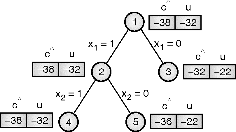
At level 2, node 4 has minimum \[ hat{c}(.) \], so it becomes E-node.
Node 6 : Inclusion of item 3 at node 4
At node 4, item 1 and 2 are already added, we have to add item 3. After including item 1, 2 and 3, item 4 cannot be accommodated. u(6) = – (10 + 10 + 12) = – 32
\[ hat{c}(6) = u(6) – frac{M – Weight ; of ; selected ; items}{Weight ; of ; remaining ; items}*Profit ; of ; remaining ; items \] \[ hat{c}(6) = -32 – frac{15 – (2 + 4 + 6)}{9}*18\] = -38
Node 7 : Exclusion of item 2 at node 2
On excluding item 3, we can accommodate item 1, 2 and 4 in knapsack.
u(7) = -(10 + 10 + 18) = – 38
\[ hat{c}(7) = u(7) – frac{M – Weight ; of ; selected ; items}{Weight ; of ; remaining ; items}*Profit ; of ; remaining ; items \] \[ hat{c}(7) = -38 – frac{15 – (2 + 4 + 9)}{6}*12\] = -38
State Space Tree:

When there is tie, we can select any node. Let’s make node 7 E-node.
Node 8 : Inclusion of item 4 at node 7
u(8) = -(10 + 10 + 18) = – 38
\[ hat{c}(8) = u(8) – frac{M – Weight ; of ; selected ; items}{Weight ; of ; remaining ; items}*Profit ; of ; remaining ; items \] \[ hat{c}(8) = -38 – frac{15 – (2 + 4 + 9)}{6}*12\] = -38
Node 9 : Exclusion of item 4 at node 7
This node excludes both the items, 3 and 4. We can add only item 1 and 2.
u(9) = -(10 + 10) = – 20
\[ hat{c}(9) = u(9) – frac{M – Weight ; of ; selected ; items}{Weight ; of ; remaining ; items}*Profit ; of ; remaining ; items \] \[ hat{c}(9) = -20 – frac{15 – (2 + 4)}{0}*0\] = -20
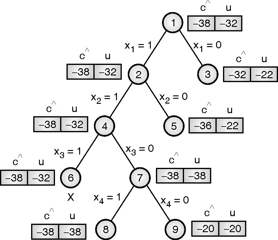
At last level, node 8 has minimum \[ hat{c}(.) \], so node 8 would be the answer node. By tracing from node 8 to root, we get item 4, 2 and 1 in the knapsack.
Solution vector X = {x1, x2, x4} and profit = p1 + p2 + p4 = 38
FIFO for Knapsack
- In FIFO branch and bound approach, variable tuple size state space tree is drawn. For each node N, cost function \[ hat{c}(.) \] and upper bound u(.) is computed similarly to the previous approach. In LC search, E node is selected from two child of current node.
- In FIFO branch and bound approach, both the children of siblings are inserted in list and most promising node is selected as new E node.
- Let us consider the same example :
Example on Knapsack Problem using Branch and Bound
Example: Solve following instance of knapsack using FIFO BB.
| i | Pi | Wi |
| 1 | 10 | 2 |
| 2 | 10 | 4 |
| 3 | 12 | 6 |
| 4 | 18 | 9 |
Solution:
Let us compute u(1) and \[ hat{c}(1) \].
u(1) = \[ sum_{}^{}p_i \] such that \[ sum w_i le M \]
= – (10 + 10 + 12) = – 32
Upper = u(1) = – 32
If we include the first three items then \[ sum w_i le M \] , but if we include 4th item, it exceeds the knapsack capacity.
\[ hat{c}(1) = u(1) – frac{M – Weight ; of ; selected ; items}{Weight ; of ; remaining ; items}*Profit ; of ; remaining ; items \] \[ hat{c}(1) = -32 – frac{15 – (2 + 4 + 6)}{9}*18\] = -38
State space tree:

Node 2 : Inclusion of item 1 at node 1
u(2) = -(10 + 10 + 12) = – 32
\[ hat{c}(2) = -32 – frac{15 – (2 + 4 + 6)}{9}*18\] = -38
Node 3 : Exclusion of item 1 at node 1
We are excluding item 1, including 2 and 3. Item 4 cannot be accommodated in a knapsack along with 2 and 3.
u(3) = -(10 + 12) = – 22
\[ hat{c}(3) = -22 – frac{15 – (4 + 6)}{9}*18\] = -32

In LC approach, node 2 would be selected as E-Node as it has minimum (×). But in FIFO approach, all child of node 2 and 3 are expanded and the most promising child becomes E-node.
Node 4 : Inclusion of item 2 at node 2
u(4) = -(10 + 10 + 12) = – 32
\[ hat{c}(4) = -32 – frac{15 – (2 + 4 + 6)}{9}*18\] = -38
Node 5 : Exclusion of item 2 at node 2
We are excluding item 1, including 2 and 3. Item 4 cannot be accommodated in a knapsack along with 2 and 3.
u(5) = -(10 + 12) = – 22
\[ hat{c}(5) = -22 – frac{15 – (4 + 6)}{9}*18\] = -32
Node 6 : Inclusion of item 2 at node 3
u(6) = -(p2 + p3) = – (10 + 12) = – 22
\[ hat{c}(6) = -22 – frac{15 – (4 + 6)}{9}*18\] = -32
Node 7 : Exclusion of item 2 at node 3
We are excluding item 1, including 2 and 3. Item 4 cannot be accommodated in a knapsack along with 2 and 3.
u(7) = -(p3 + p4) = – (12 + 18) = – 30
\[ hat{c}(7) = -30 – 0 \] = -30

Out of node 4, 5, 6 and 7, \[ hat{c}(7) \] > upper, so kill node 7. Remaining 3 nodes are live and added in list. Out of 4, 5 and 6, node 4 has minimum \[ hat{c} \] value, so it becomes next E-node.
Node 8 : Inclusion of item 3 at node 4
u(8) = -(10 + 10 + 12) = – 32
\[ hat{c}(8) = -32 – frac{15 – (2 + 4 + 6)}{9}*18\] = -38
Node 9 : Exclusion of item 3 at node 4
We are excluding item 3, including 1 and 2 and 4.
u(9) = -(p1 + p2 + p4) = – (10 + 10 + 18) = – 38
\[ hat{c}(9) = -38 – 0 \] = -38
Upper = u(9) = – 38.
\[ hat{c}(5) \] > upper and \[ hat{c}(6) \] > upper, so kill them. If we continue in this way, final state space tree looks as follow :

Node 12 has minimum cost function value, so it will be the answer node.
Solution vector = {x1, x2, x4},
profit = 10 + 10 + 18 = 38