Merge Sort

Merge sort sorts the list using divide and conquers strategy. Unlike selection sort, bubble sort or insertion sort, it sorts data by dividing the list into sub lists and recursively solving and combining them.

It works on following two basic principles :

• Sorting a smaller list takes less time than sorting a larger list.
• Combining two sorted sublists takes less time than combining two unsorted lists.

Merge sort works in three stages :

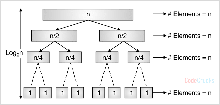
• Divide : Recursively divide the single list into two sublists until each sublist contains 1 element.
• Conquer : Sort both sublists of parent list. List of 1 element is sorted.
• Combine : Recursively combine sorted sublists until the list of size n is produced.

Merge sort divides the list of size n into two sublists, each of size n/2. This subdivision continues until problem size becomes one. After hitting to the problem size one, conquer phase starts. Following figure shows the divide phase.

Two Way Merge

Two-way merge is the process of merging two sorted arrays of size m and n into a single sorted array of size (m + n).

Merge sort compares two arrays, each of size one, using a two-way merge. The sorted sequence is saved in a new two-dimensional array. In the following step, two sorted arrays of size two are combined to form a single sorted array of size four. This technique is repeated until the entire problem has been solved.

To inform the algorithm that all elements in the referenced array have been examined, a sentinel symbol is added at the end of both arrays to be merged. When one array reaches to its sentinel symbol, the remaining elements of other array are simply duplicated into the final array.

Simulation of two way merge is shown in following figure.

Image Source: https://blog.shahadmahmud.com/merge-sort/ [link]

Algorithm of Merge Sort

Algorithm MERGE_SORT(A, low, high)
// Description : Sort elements of array A using Merge sort 
// Input : Array of size n, low ← 1 and  high ← n
// Output : Sorted array B

if low < high then
  mid ← floor(low + high) / 2   
  MERGE_SORT(A, low, mid)        
  MERGE_SORT (A, mid + 1, high)  
  COMBINE(A, low, mid, high)   // Merge two sorted sub lists
end

COMBINE is a two-way merge procedure that creates a sorted array of size n from two sorted arrays of size n /2. The following is how the subroutine works:

COMBINE(A, low, mid, high)

l1 ← mid – low + 1	// Size of 1starray
l2 ← high – mid		// Size of 2ndarray

for i ← 1 to l1 do
  LEFT [i] ← A [low + i–1]   
end

for j ← 1 to l2 do
  RIGHT [j] ← A [mid + j]
end

// Insert sentinel symbol at the end of each array
LEFT [l1 + 1] ← ∞
RIGHT [l2 +  1] ← ∞		

// Start two-way merge process
i ← 1, j ← 1
for k ← low to high do
  if LEFT [i] ≤ RIGHT [j] then
    B[k] ← LEFT [i]
    i ← i + 1	
  else
    B[k] ← RIGHT[j]
    j ← j + 1	
  end 
end

Complexity Analysis

• On each recursive call, the list is divided into two sublists, and problem size reduces by half. After sorting two sublists of size (n / 2), combine procedure takes n comparisons to form the sorted list of size n. Total running time of merge sort is computed by summing complexity of following three steps:
• Divide : This step computes the middle index of the array, which can be done in constant time. Thus,
  D(n) = Q(1).
• Conquer : We recursively solve two subproblems, each of size (n / 2), which contributes 2T(n/2) to the running time.
• Combine : COMBINE procedure merges two sublists, each of size n/2 and does n comparisons, thus
  C(n) = Q(n).
• Hence, T(n) = T(Conquer) + T(Divide) + T(Combine)

T(n) = 0, if n = 1

T(n) = T(n/2) + T(n/2) + D(n) + C(n), if n > 1

The first T(n/2) = Cost for solving left sub list

The second T(n/2) = Cost for solving right sub list

D(n) is cost of division, which is constant, i.e. O(1) as the list splitting is done simply by computing the middle of the array

C(n) is cost of conquer, which is linear, i.e. O(n) as two sub lists each of size n/2 are merged into bigger sorted array of size n with the help of maximum n comparisons

So, T(n) = 2T(n/2) + O(1) + O(n)

T(n) = 2T(n/2) + n … (1)

We will derive the time complexity of merge sort using two methods:

• Substitution method
• Master method

Substitution method:

Solving original recurrence for n/2,

T(n/2) = 2T(n/4) + n/2

Substituting this in equation (1),

T(n) = 2[ 2T(n/4) + n/2 ] + n

= 2² T(n/2²) + 2n

.

.

.

After k substitutions,

T(n) = 2^k T(n/2^k) + k.n … (2)

Division of array creates binary tree, which has height log₂n, so let us consider that k grows up to log₂n,

k = log₂n ⇒ n = 2^k

Substitute these values in equation (2)

T(n) = nT(n/n) + log₂n . n

T(n) = O(n.log₂n) (because, T(1) = 0, from base case)

Master method:

Recurrence of the merge sort, T(n) = 2T(n/2) + n is of the form T(n) = a.T(n/b) + f(n),

Comparing both the recurrence,

a = 2, b = 2 and f(n) = n with d = 1, where d is the degree of polynomial function f(n).

b^d = 2¹ = 2 Here, a = b^d, so from the Case 1 of Variant – I of master method,

T(n) = O(n^dlog₂n)

= O(nlog₂n)

Whether the list is already sorted, inverse sorted or randomly shuffled, all three steps must be performed. Merge sort cannot detect if the list is sorted. So numbers of comparisons are the same for all three cases. The time complexity of algorithm for all three cases is stated in the following table :

Best case	Average case	Worst case
O(nlog2n)	O(nlog2n)	O(nlog2n)

Running time of this algorithm is similar to heap sort method.

Examples of Merge Sort

Problem: Simulate merge sort on data sequence <77, 22, 33, 44, 11, 55, 66>

Solution:

Let us understand the working of merge sort through graphical representation and call sequences. Consider the sequence of the element as shown below

Simulation of merge sort for the given array is depicted in following figure. The number in a circle on the left or right corner indicates the call sequence. COMBINE is called as soon as two sublists of size 1 are created.

Let us see how COMBINE does a two-way merge of two arrays. Consider the two sorted sublists
LEFT = {22, 33, 44, 77} and RIGHT = {11, 55, 66}.

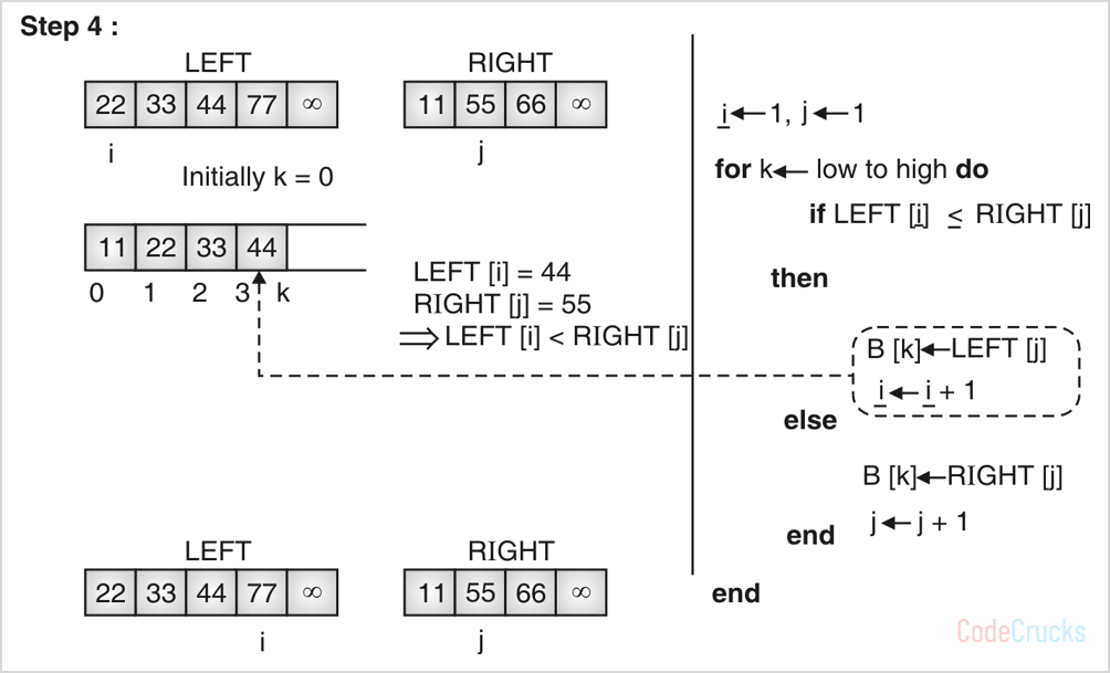
Finally, the sorted sequence of two sub lists LEFT = {22, 33, 44, 77} and RIGHT = {11, 55, 66} would be B={11, 22, 33, 44, 55, 66, 77}

Problem: Sort the sequence using a merge sort algorithm : A { 33, 22, 44, 00, 99, 88, 11 }

Solution:

Merge sort works as follow :

Algorithm MERGE_SORT (A, low, high)
if low < high then 
  mid ← (low + high) / 2
  MERGE_SORT (A, low, mid)
  MERGE_SORT (A, mid +1, high)
  COMBINE (A, low, mid, high)
end

Variable low and high represents the first and last index of the passed array. Call sequence is shown in following figure

From the above pseudo-code, we can see that no two calls are parallel. Each call is one of the three calls made in MERGE_SORT(A, low, high) procedure stated above. Calling sequence for given data is shown below (according to the picture, low = 0, high = 6) :

The number beside the dotted line indicates call number in the entire sequence of merge sort procedure. Call sequence for a given example is shown below:

Step-0:    MERGE_SORT(A, 0, 6)

Step-1:    MERGE_SORT(A, 0, 3)

Step-2:    MERGE_SORT(A, 0, 1)

Step-3:    MERGE_SORT(A, 0, 0)

Step-4:    MERGE_SORT(A, 1, 1)

Step-5:    COMBINE(A, 0, 0, 1)

Step-6:    MERGE_SORT(A, 2, 3)

Step-7:    MERGE_SORT(A, 2, 2)

Step-8:    MERGE_SORT(A, 3, 3)

Step-9:    COMBINE (A, 2, 2, 3)

Step-10:  COMBINE (A, 0, 1, 3)

Step-11:  MERGE_SORT(A, 4, 6)

Step-12:  MERGE_SORT(A, 4, 5)

Step-13:  MERGE_SORT(A, 4, 4)

Step-14:  MERGE_SORT(A, 5, 5)

Step-15:  COMBINE (A, 4, 4, 5)

Step-16:  MERGE_SORT(A, 6, 6)

Step-17:  COMBINE (A, 4, 5, 6)

Step-18: COMBINE (A, 0, 3, 6)

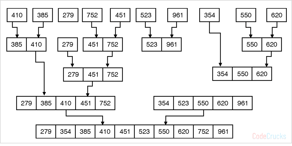
Problem: Sort the following elements: 410, 385, 279, 752, 451, 523, 961, 354, 550, 620

Solution:

Algorithm first divides the list into two halves. Splitting is continuing until problem size reaches to 1.

We computed the mid value as follow :

mid = ceil(low + high) / 2

rather than,

mid = floor(low + high) / 2

Divide phase for given data is described in following figure

When problem size becomes trivial (i.e. n = 1), the algorithm starts solving the problem and merging solutions of smaller subproblems. The solution is constructed in a bottom-up approach. Conquer procedure is illustrated in following figure:

Simulation

Step by step simulation of sorting process is shown in following animation

Image Source: https://en.wikipedia.org/wiki/Merge_sort

Properties of Merge Sort

• Not Adaptive: Running time of it does not change with input sequence.
• Stable / Unstable: Both implementations are possible.
• Not Incremental: Does not sort one by one element in each pass, so it is not incremental.
• Not online: Need all data to be in memory at the time of sorting, so it is not online.
• Not in place: It needs O(n) extra space to sort two sublists of size (n / 2).

Some Popular Sorting Algorithms

Following are the few popular sorting algorithms used in computer science:

• Bubble sort
• Selection sort
• Insertion sort
• Heap sort
• Merge sort
• Quick sort
• Counting sort
• Radix sort
• Bucket sort